Overview
This vignette is an introduction to the usage of pareg. It estimates pathway enrichment scores by regressing differential expression p-values of all genes considered in an experiment on their membership to a set of biological pathways. These scores are computed using a regularized generalized linear model with LASSO and network regularization terms. The network regularization term is based on a pathway similarity matrix (e.g., defined by Jaccard similarity) and thus classifies this method as a modular enrichment analysis tool (Huang, Sherman, and Lempicki 2009).
Installation
if (!require("BiocManager", quietly = TRUE)) {
  install.packages("BiocManager")
}
BiocManager::install("pareg")
Load required packages
We start our analysis by loading the pareg package and other required libraries.
Introductory example
Generate pathway database
For the sake of this introductory example, we generate a synthetic pathway database with a pronounced clustering of pathways.
group_num <- 2
pathways_from_group <- 10

gene_groups <- purrr::map(seq(1, group_num), function(group_idx) {
  glue::glue("g{group_idx}_gene_{seq_len(15)}")
})
genes_bg <- paste0("bg_gene_", seq(1, 50))

df_terms <- purrr::imap_dfr(
  gene_groups,
  function(current_gene_list, gene_list_idx) {
    purrr::map_dfr(seq_len(pathways_from_group), function(pathway_idx) {
      data.frame(
        term = paste0("g", gene_list_idx, "_term_", pathway_idx),
        gene = c(
          sample(current_gene_list, 10, replace = FALSE),
          sample(genes_bg, 10, replace = FALSE)
        )
      )
    })
  }
)

df_terms %>%
  sample_n(5)
## term gene
## 1 g1_term_9 g1_gene_12
## 2 g1_term_5 g1_gene_7
## 3 g2_term_2 g2_gene_2
## 4 g1_term_3 bg_gene_47
## 5 g1_term_8 g1_gene_1Term similarities
Before starting the actual enrichment estimation, we compute pairwise pathway similarities with pareg’s helper function.
mat_similarities <- compute_term_similarities(
  df_terms,
  similarity_function = jaccard
)

hist(mat_similarities, xlab = "Term similarity")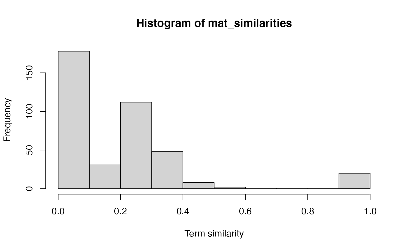
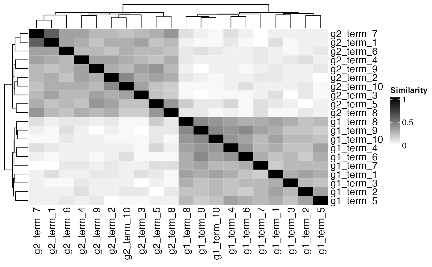
We can see a clear clustering of pathways.
Heatmap(
  mat_similarities,
  name = "Similarity",
  col = circlize::colorRamp2(c(0, 1), c("white", "black"))
)
Create synthetic study
We then select a subset of pathways to be activated. In a performance evaluation, these would be considered to be true positives.
active_terms <- similarity_sample(mat_similarities, 5)
active_terms
## [1] "g2_term_6" "g2_term_3" "g2_term_3" "g2_term_2" "g2_term_8"The genes contained in the union of active pathways are considered to be differentially expressed.
de_genes <- df_terms %>%
  filter(term %in% active_terms) %>%
  distinct(gene) %>%
  pull(gene)

other_genes <- df_terms %>%
  distinct(gene) %>%
  pull(gene) %>%
  setdiff(de_genes)
The p-values of genes considered to be differentially expressed are sampled from a Beta distribution centered at \(0\). The p-values for all other genes are drawn from a Uniform distribution.
df_study <- data.frame(
  gene = c(de_genes, other_genes),
  pvalue = c(rbeta(length(de_genes), 0.1, 1), rbeta(length(other_genes), 1, 1)),
  in_study = c(
    rep(TRUE, length(de_genes)),
    rep(FALSE, length(other_genes))
  )
)

table(
  df_study$pvalue <= 0.05,
  df_study$in_study, dnn = c("sig. p-value", "in study")
)
## in study
## sig. p-value FALSE TRUE
## FALSE 34 17
## TRUE 1 28Enrichment analysis
Finally, we compute pathway enrichment scores.
fit <- pareg(
  df_study %>% select(gene, pvalue),
  df_terms,
  network_param = 1, term_network = mat_similarities
)
## Loaded Tensorflow version 2.3.0The results can be exported to a dataframe for further processing…
| term | enrichment |
|---|---|
| g2_term_6 | -0.6760687 |
| g2_term_3 | -0.6005415 |
| g2_term_2 | -0.5818557 |
| g2_term_4 | -0.4233026 |
| g2_term_8 | -0.4123425 |
| g1_term_2 | 0.3978593 |
…and also visualized in a pathway network view.
plot(fit, min_similarity = 0.1)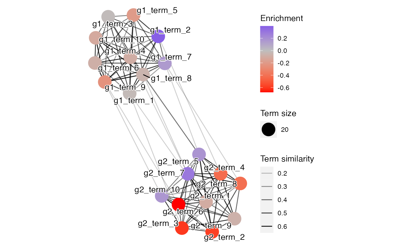
To provide a wider range of visualization options, the result can be transformed into an object which is understood by the functions of the enrichplot package.
obj <- as_enrichplot_object(fit)

dotplot(obj) +
  scale_colour_continuous(name = "Enrichment Score")
## Scale for 'colour' is already present. Adding another scale for 'colour',
## which will replace the existing scale.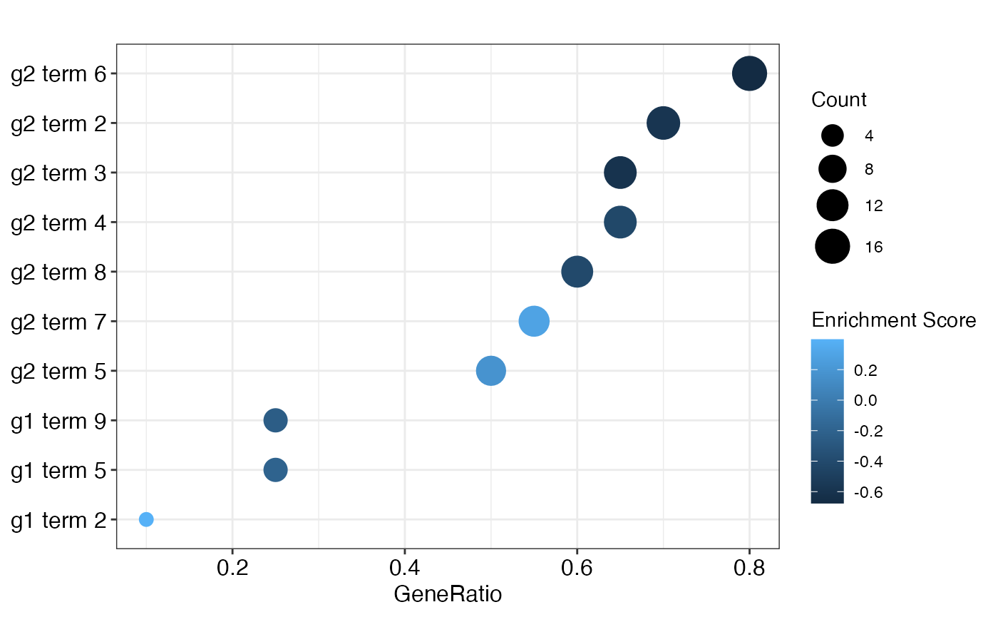
treeplot(obj) +
  scale_colour_continuous(name = "Enrichment Score")
## Scale for 'colour' is already present. Adding another scale for 'colour',
## which will replace the existing scale.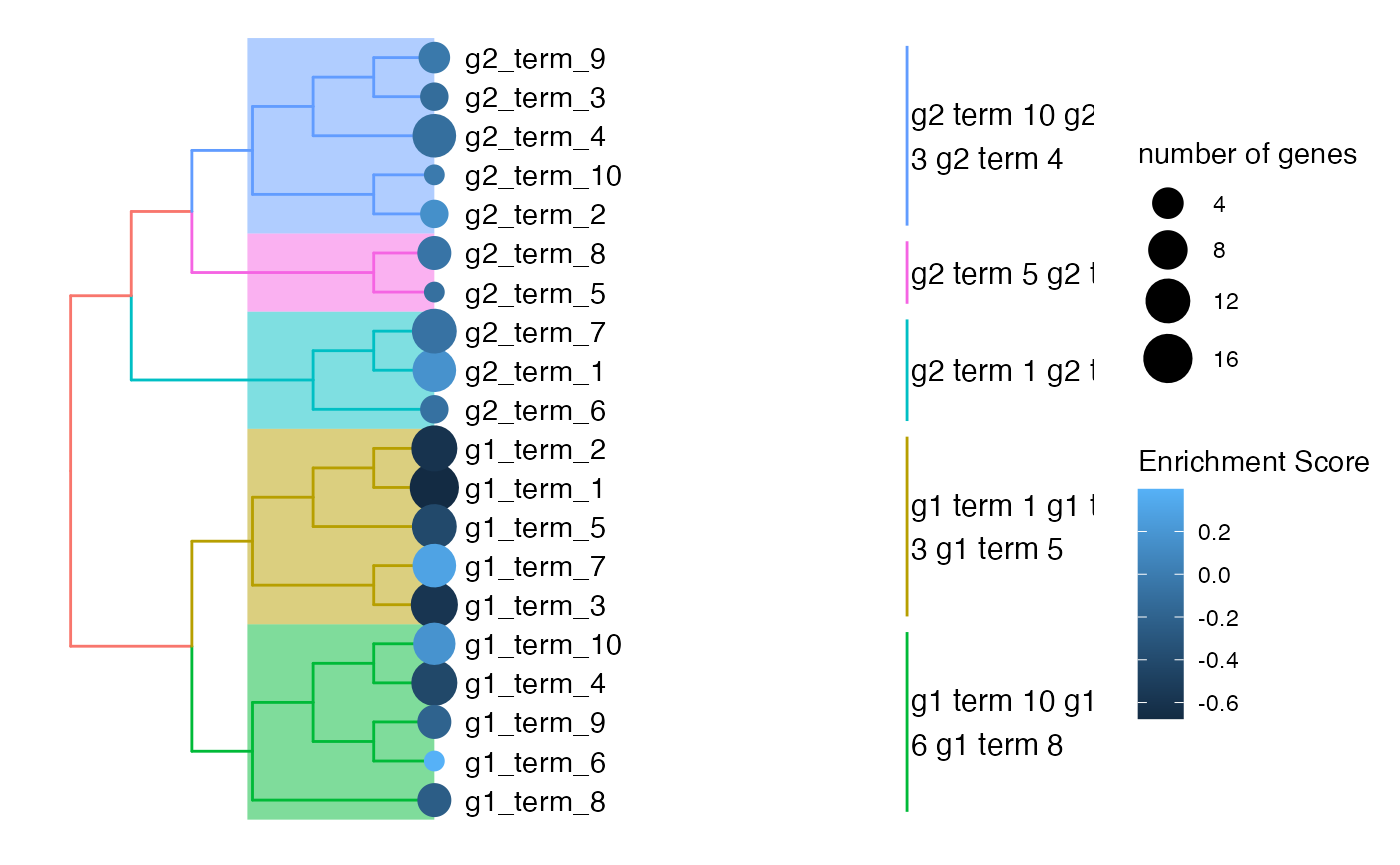
Session information
## R version 4.2.1 (2022-06-23)
## Platform: x86_64-apple-darwin17.0 (64-bit)
## Running under: macOS Big Sur ... 10.16
##
## Matrix products: default
## BLAS:   /Library/Frameworks/R.framework/Versions/4.2/Resources/lib/libRblas.0.dylib
## LAPACK: /Library/Frameworks/R.framework/Versions/4.2/Resources/lib/libRlapack.dylib
##
## locale:
## [1] en_US.UTF-8/en_US.UTF-8/en_US.UTF-8/C/en_US.UTF-8/en_US.UTF-8
##
## attached base packages:
## [1] grid      stats     graphics  grDevices utils     datasets  methods
## [8] base
##
## other attached packages:
##  [1] pareg_0.99.5          tfprobability_0.15.0  tensorflow_2.9.0
##  [4] enrichplot_1.16.1     ComplexHeatmap_2.12.0 forcats_0.5.1
##  [7] stringr_1.4.0         dplyr_1.0.9           purrr_0.3.4
## [10] readr_2.1.2           tidyr_1.2.0           tibble_3.1.7
## [13] tidyverse_1.3.1       ggraph_2.0.5          ggplot2_3.3.6
## [16] BiocStyle_2.24.0
##
## loaded via a namespace (and not attached):
##   [1] utf8_1.2.2             reticulate_1.25-9000   tidyselect_1.1.2
##   [4] RSQLite_2.2.14         AnnotationDbi_1.58.0   BiocParallel_1.30.3
##   [7] devtools_2.4.3         scatterpie_0.1.7       munsell_0.5.0
##  [10] codetools_0.2-18       ragg_1.2.2             future_1.26.1
##  [13] withr_2.5.0            keras_2.9.0            colorspace_2.0-3
##  [16] GOSemSim_2.22.0        Biobase_2.56.0         highr_0.9
##  [19] logger_0.2.2           knitr_1.39             rstudioapi_0.13
##  [22] stats4_4.2.1           DOSE_3.22.0            listenv_0.8.0
##  [25] labeling_0.4.2         GenomeInfoDbData_1.2.8 polyclip_1.10-0
##  [28] bit64_4.0.5            farver_2.1.0           rprojroot_2.0.3
##  [31] parallelly_1.32.0      vctrs_0.4.1            treeio_1.20.0
##  [34] generics_0.1.3         xfun_0.31              R6_2.5.1
##  [37] doParallel_1.0.17      GenomeInfoDb_1.32.2    clue_0.3-61
##  [40] graphlayouts_0.8.0     bitops_1.0-7           cachem_1.0.6
##  [43] fgsea_1.22.0           gridGraphics_0.5-1     assertthat_0.2.1
##  [46] scales_1.2.0           gtable_0.3.0           globals_0.15.1
##  [49] processx_3.6.1         tidygraph_1.2.1        rlang_1.0.3
##  [52] zeallot_0.1.0          systemfonts_1.0.4      GlobalOptions_0.1.2
##  [55] splines_4.2.1          lazyeval_0.2.2         broom_1.0.0
##  [58] BiocManager_1.30.18    yaml_2.3.5             reshape2_1.4.4
##  [61] modelr_0.1.8           backports_1.4.1        qvalue_2.28.0
##  [64] usethis_2.1.6          tools_4.2.1            bookdown_0.27
##  [67] ggplotify_0.1.0        ellipsis_0.3.2         jquerylib_0.1.4
##  [70] RColorBrewer_1.1-3     proxy_0.4-27           BiocGenerics_0.42.0
##  [73] sessioninfo_1.2.2      Rcpp_1.0.8.3           plyr_1.8.7
##  [76] progress_1.2.2         base64enc_0.1-3        zlibbioc_1.42.0
##  [79] RCurl_1.98-1.7         ps_1.7.1               prettyunits_1.1.1
##  [82] GetoptLong_1.0.5       viridis_0.6.2          S4Vectors_0.34.0
##  [85] haven_2.5.0            ggrepel_0.9.1          cluster_2.1.3
##  [88] here_1.0.1             fs_1.5.2               magrittr_2.0.3
##  [91] data.table_1.14.2      DO.db_2.9              circlize_0.4.15
##  [94] reprex_2.0.1           whisker_0.4            ggnewscale_0.4.7
##  [97] matrixStats_0.62.0     pkgload_1.3.0          hms_1.1.1
## [100] patchwork_1.1.1        evaluate_0.15          readxl_1.4.0
## [103] IRanges_2.30.0         gridExtra_2.3          shape_1.4.6
## [106] tfruns_1.5.0           compiler_4.2.1         crayon_1.5.1
## [109] shadowtext_0.1.2       htmltools_0.5.2        ggfun_0.0.6
## [112] tzdb_0.3.0             aplot_0.1.6            lubridate_1.8.0
## [115] DBI_1.1.3              tweenr_1.0.2           dbplyr_2.2.1
## [118] MASS_7.3-57            Matrix_1.4-1           cli_3.3.0
## [121] parallel_4.2.1         igraph_1.3.2           pkgconfig_2.0.3
## [124] pkgdown_2.0.5          xml2_1.3.3             foreach_1.5.2
## [127] ggtree_3.4.0           bslib_0.3.1            rngtools_1.5.2
## [130] XVector_0.36.0         doFuture_0.12.2        rvest_1.0.2
## [133] doRNG_1.8.2            yulab.utils_0.0.5      callr_3.7.0
## [136] digest_0.6.29          Biostrings_2.64.0      rmarkdown_2.14
## [139] cellranger_1.1.0       fastmatch_1.1-3        tidytree_0.3.9
## [142] nloptr_2.0.3           rjson_0.2.21           lifecycle_1.0.1
## [145] nlme_3.1-157           jsonlite_1.8.0         desc_1.4.1
## [148] viridisLite_0.4.0      fansi_1.0.3            pillar_1.7.0
## [151] lattice_0.20-45        KEGGREST_1.36.2        fastmap_1.1.0
## [154] httr_1.4.3             pkgbuild_1.3.1         GO.db_3.15.0
## [157] remotes_2.4.2          glue_1.6.2             png_0.1-7
## [160] iterators_1.0.14       bit_4.0.4              ggforce_0.3.3
## [163] stringi_1.7.6          sass_0.4.1             blob_1.2.3
## [166] textshaping_0.3.6      memoise_2.0.1          ape_5.6-2